
EpiScout™ Analysis Software
Detect, locate, and quantify multiple RNA modifications plus RNA expression with the EpiScout Analysis Pipeline.
Provided below are links to publicly accessible EpiPlex data generated from human peripheral blood mononuclear cell (PBMC) and liver tissue RNA. Please scroll down on the page for a step-by-step introduction to some of the EpiScout analyses.
View an example report
View Report
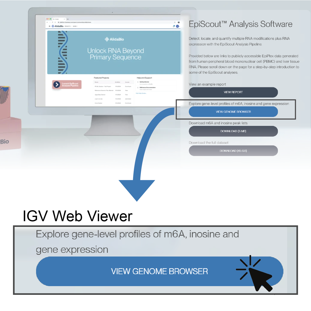
Explore gene-level profiles of m6A, inosine and gene expression
View Genome Browser
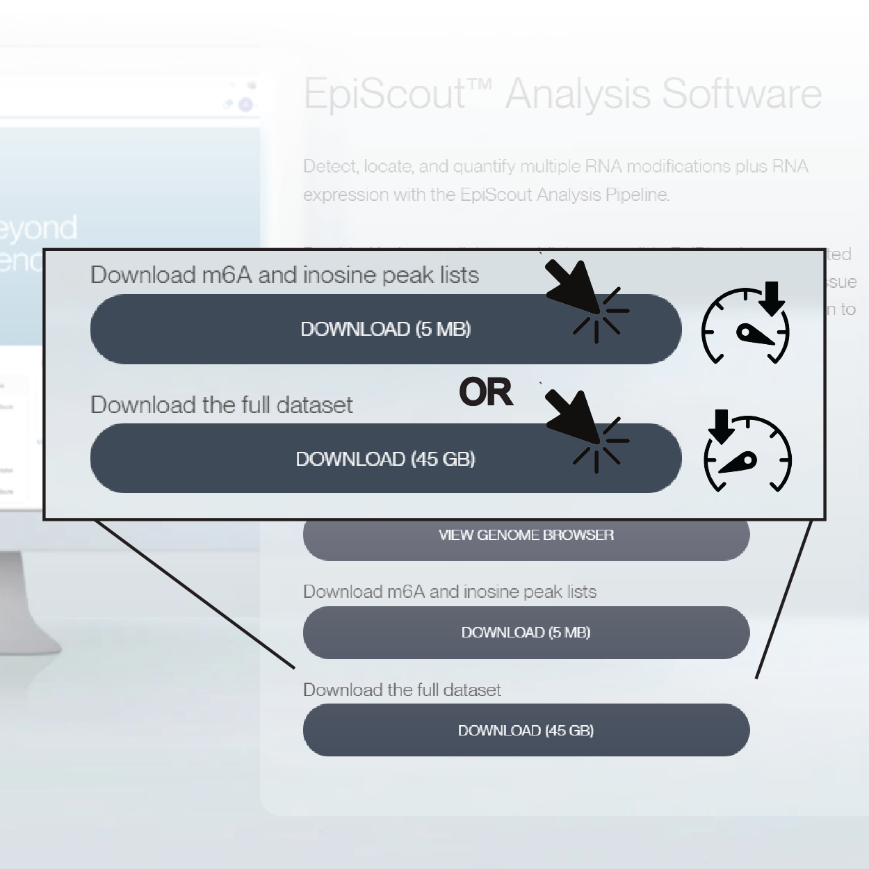
Download m6A and inosine peak lists
Download (5 Mb)
Download the full dataset
Download (45 Gb)

Tutorial: Exploring EpiScout Data
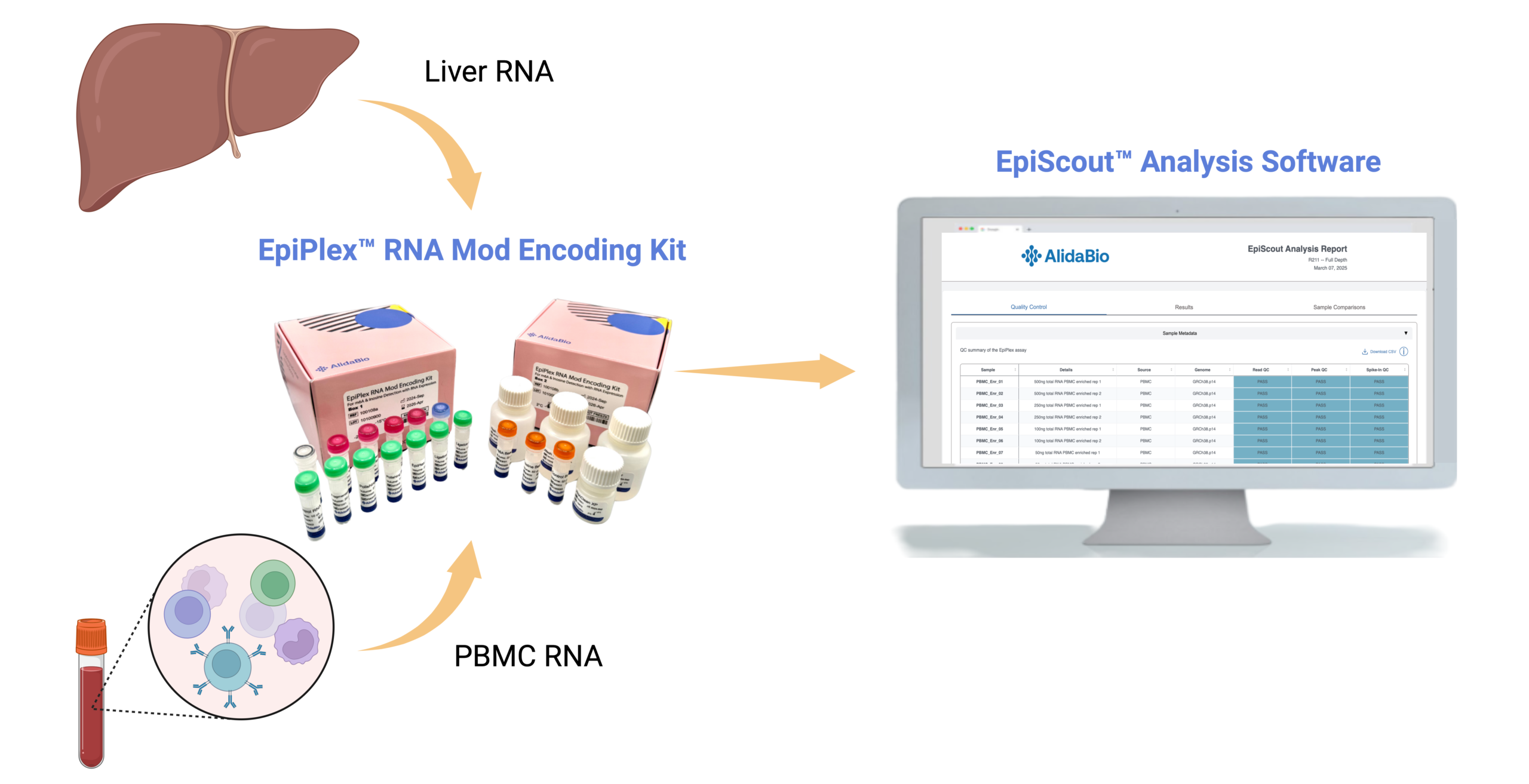
This publicly available dataset was generated using RNA extracted from human peripheral blood mononuclear cells (PBMC) and liver tissue sourced from BioChain Institute Inc. Modification-enriched and RNA-Seq libraries were generated in duplicate for each sample using the EpiPlex Total RNA workflow. The assay detects both N6-methyladenosine (m6A) and inosine in a single run, while also producing high-quality RNA-Seq data from a matched solution control.
Getting Started
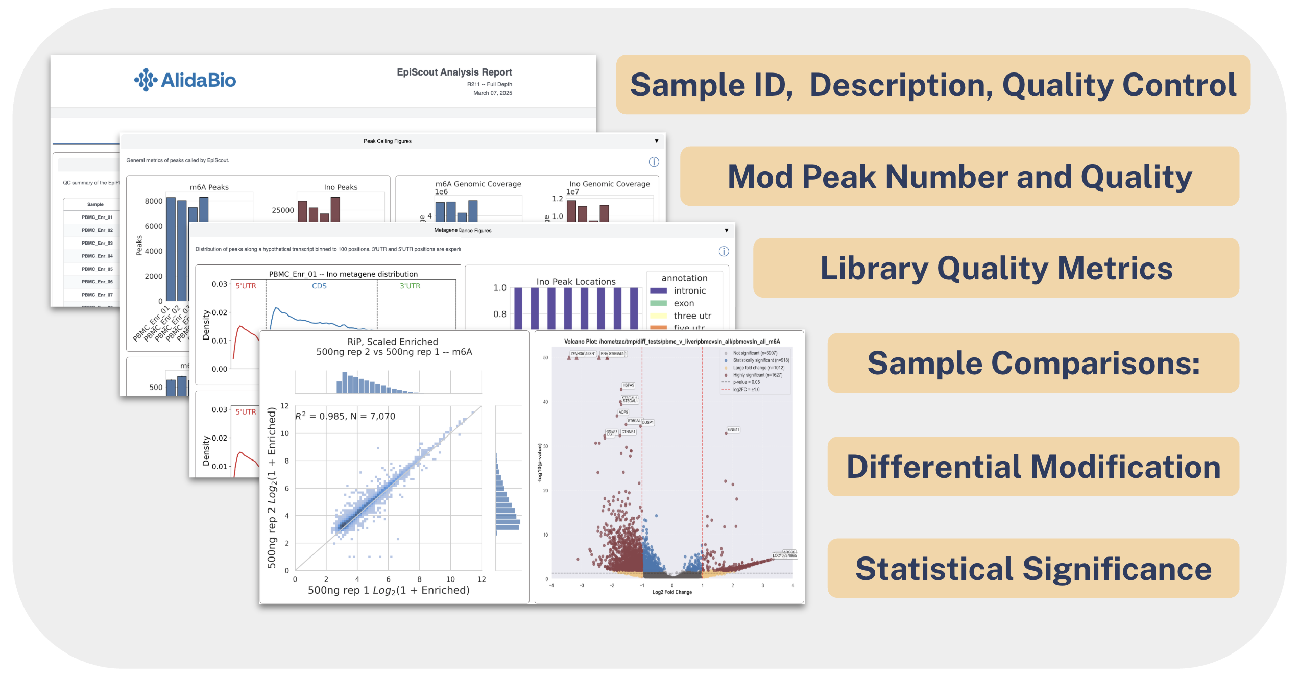
The EpiScout Analysis Software provides a suite of outputs that make it easy to find biologically interesting signals. As with any large dataset, the best starting point is a high-level overview to confirm data quality before drilling into specific genes or regions. In an EpiScout run, this overview comes from the interactive EpiScout Analysis Report, viewable in any web browser.
A report generated from this PBMC and liver experiment can be accessed below:
Validating Experimental Data
The first tab of the EpiScout report presents high-level quality control metrics. The color coding allows you to quickly gauge experimental performance.
EpiScout Report
Quality Control Overview
Parameter values are conveniently colored to quickly identify values outside of the expected range.
Blue: value is within expected range
Yellow: value is potentially out of range, but may be sample-type specific
Red: value is significantly out of range, please contact support
Important Metrics to Consider:
- Total reads enriched or solution control: > 15M
- Mapped reads: > 70%
- m6A reads: > 8M
- Inosine reads > 2M
- Duplication rate: < 50%
- m6A peaks containing DRACH: > 80%
- Inosine peaks containing A-to-G: > 85%
Interpret these ranges alongside project context and replicate consistency.
Investigating Your Genes of Interest
It can be difficult to know where to start when working with large datasets. One of the best ways to start navigating through data is to start with the most highly modified genes and regions in the sample. These regions are often cell-type specific, and can act as a point of reference for characteristics of intense and confident signal. You can locate these modified regions in a given sample by looking at its peak list. An example peak list can be found below:
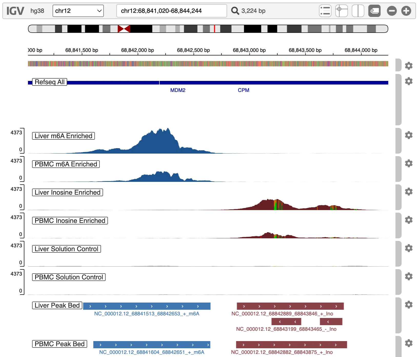
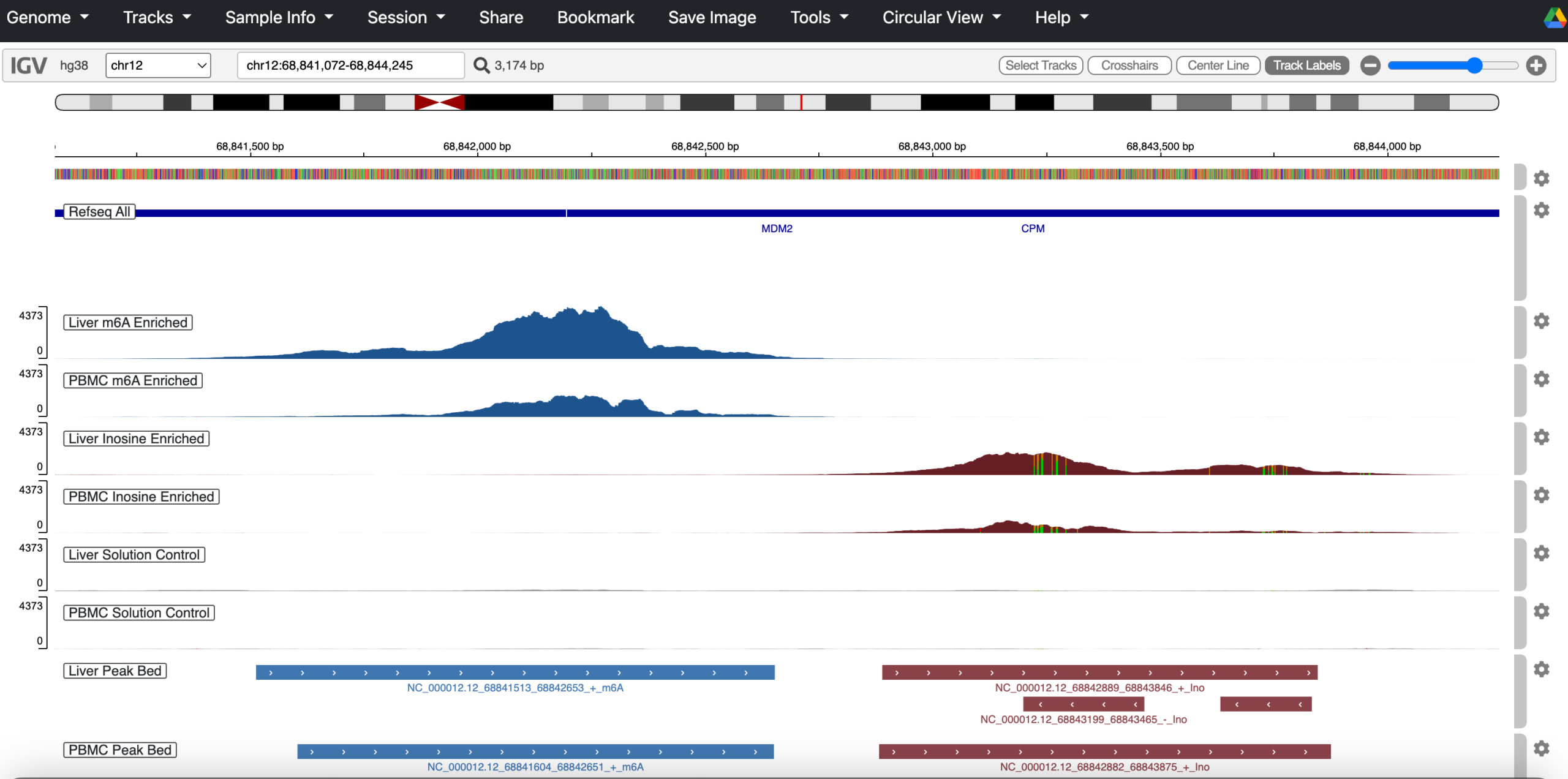
Once you have a specific peak or region of interest, the next step would be to check this transcript at the gene-level. Read pileups offer a raw but informative view of RNA modification landscapes, providing visual insight into how heavily modified a given region is. They’re especially useful for spotting co-localization between m⁶A and inosine peaks. A compelling example is visible in the 3′UTR of the MDM2 gene, which appears immediately when you launch the genome browser:
Quick Start Guide for Finding Modified Regions of Interest with a Genome Browser
1. Download the peak list or full data set
Links to the m6A and inosine peak lists are available for download. The peak lists contain relevant gene information associated with the modified regions of interest. This includes the coordinates and intensity of each peak, gene feature annotations, and statistical confidence and known molecular patterns.
Alternately, download the full dataset which also contains the peak lists.
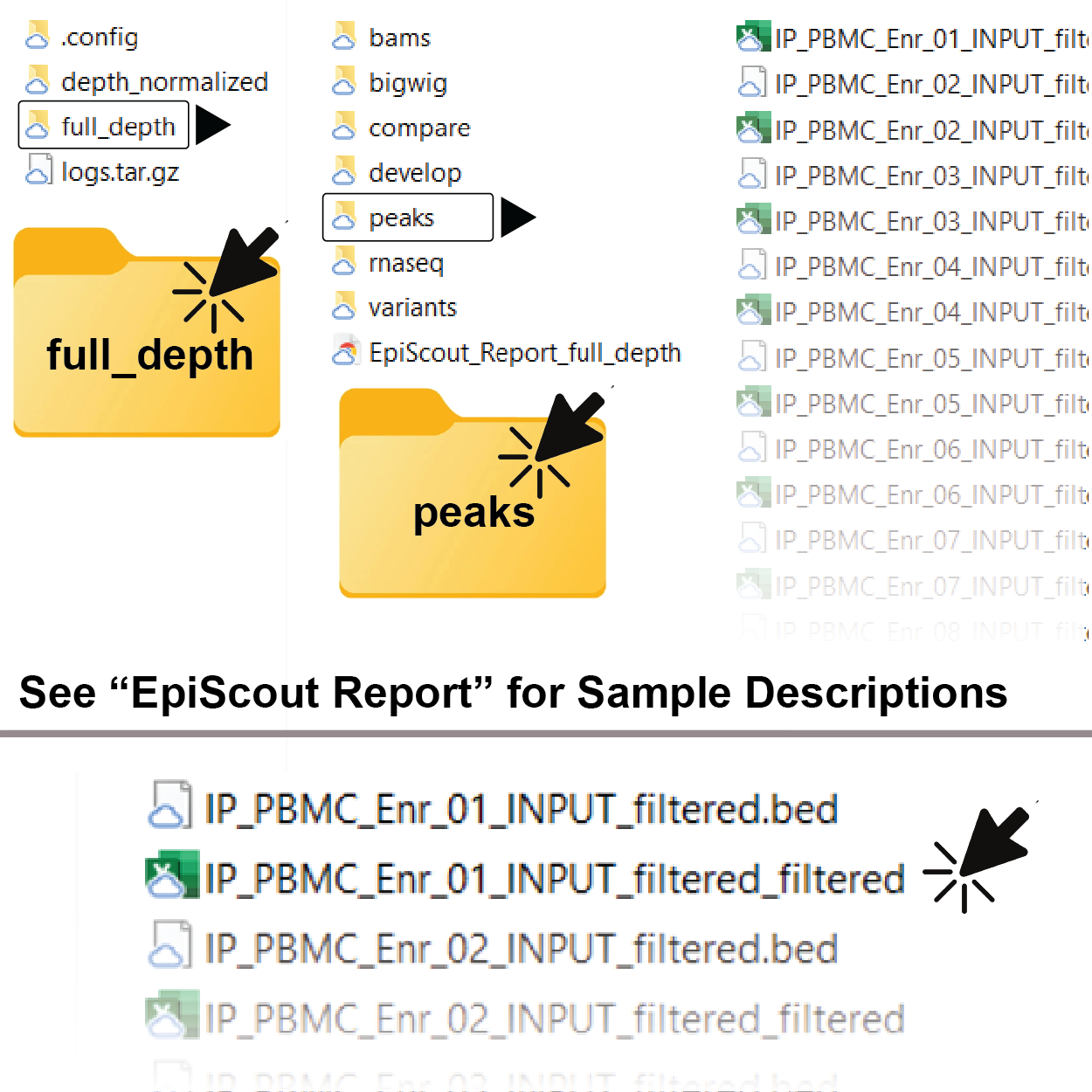
2. Navigate to and Open the Peak.tsv file
If you downloaded the full dataset, you will need to unzip the file and then navigate to the “full_depth” directory. You can then find the peak lists in the “peaks” folder. The peak lists are .tsv files and can be opened in Microsoft Excel, Google Sheets, or any other spreadsheet software.
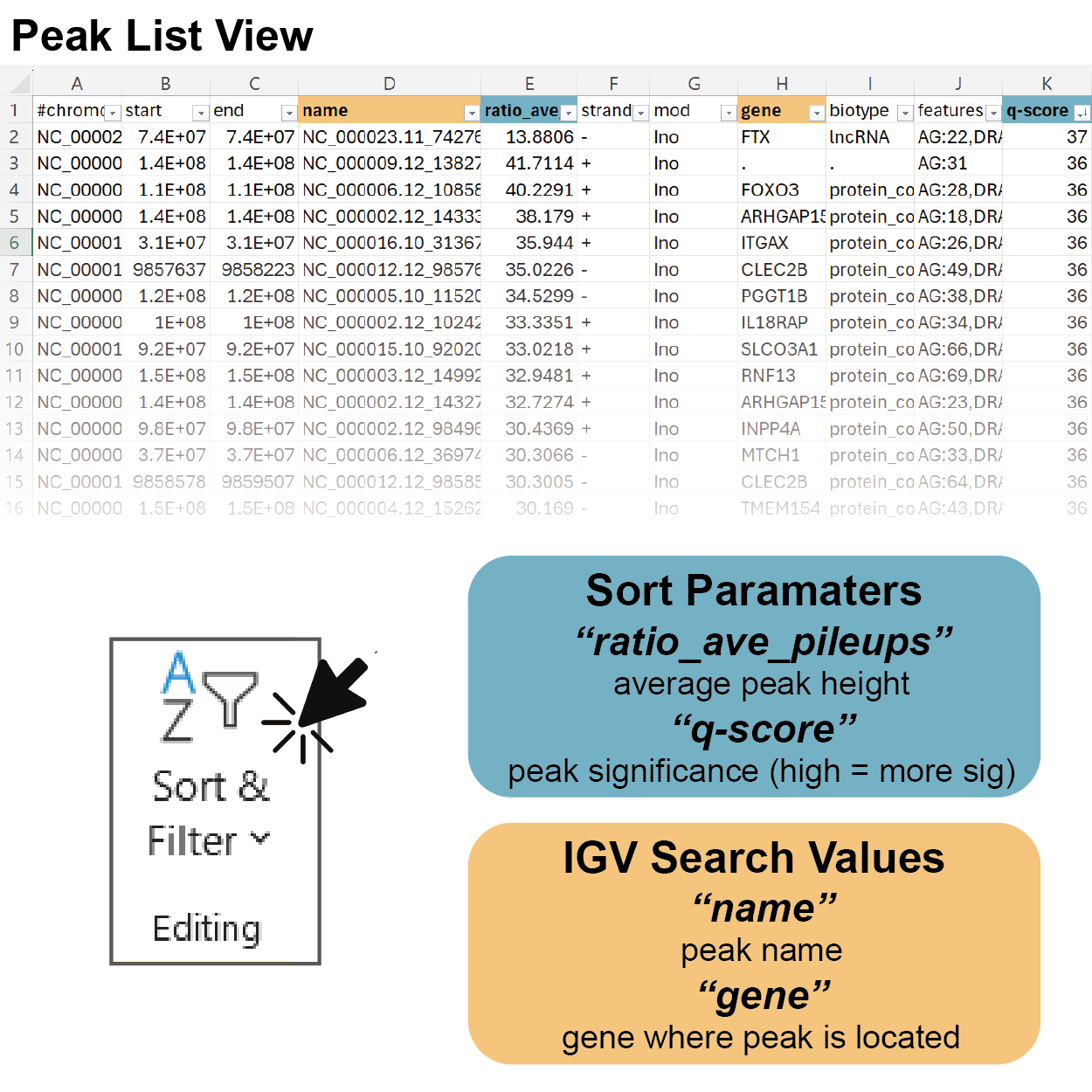
3. Sort the Peak Table by Your Parameter of Interest
Peak intensity is calculated as a “ratio_ave_pileup” value which takes into account the average read pileup of the modification enriched channel and paired RNASeq channel across a given region of interest defined by the peak coordinates. Sorting by this value will show you the gene regions which are most highly modified relative to native gene expression.
4. Open a Genome Browser to Inspect Peaks at the Gene-level
Read pileups offer a raw but informative view of RNA modification landscapes, providing visual insight into how heavily modified a given region is. They’re especially useful for spotting co-localization between m⁶A and inosine peaks. A compelling example is visible in the 3′UTR of the MDM2 gene, which appears immediately when you launch the genome browser.
To explore these patterns yourself, use the link above to open the genome browser with pre‑loaded .bam files. This allows you to visually inspect aligned reads and assess peak features corresponding to entries in the provided peak list.
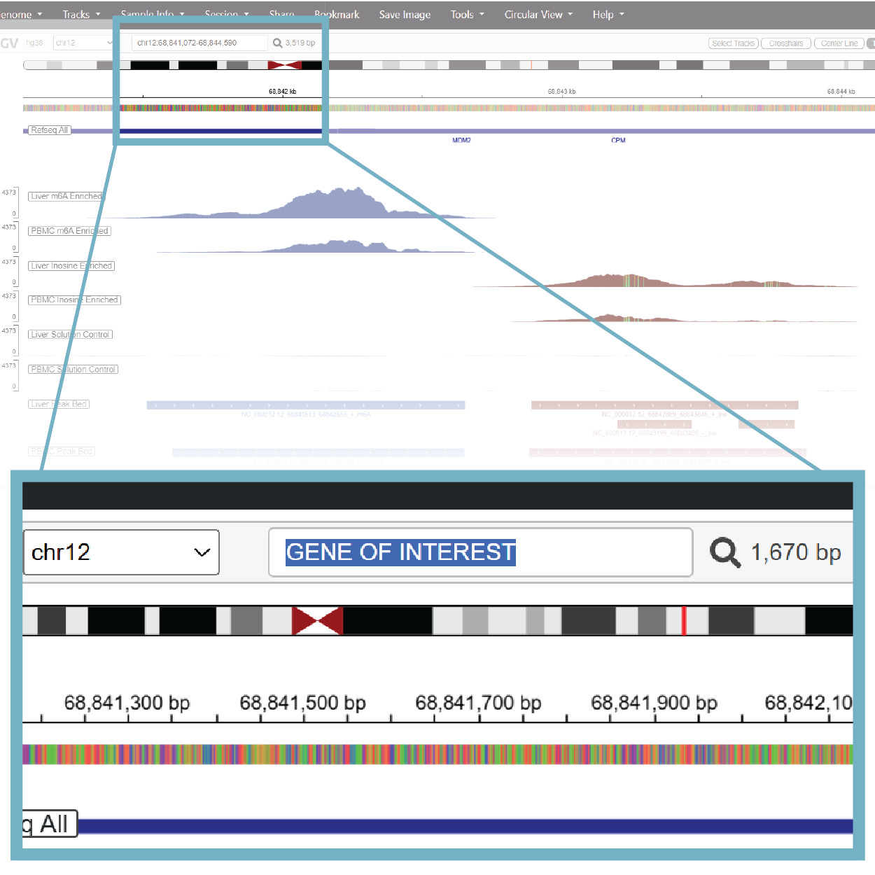
5. Use the Search Bar to Navigate to Other Genes
The search bar will take gene names or genomic coordinates. Simply type them into the box and the browser will load into your region of interest.
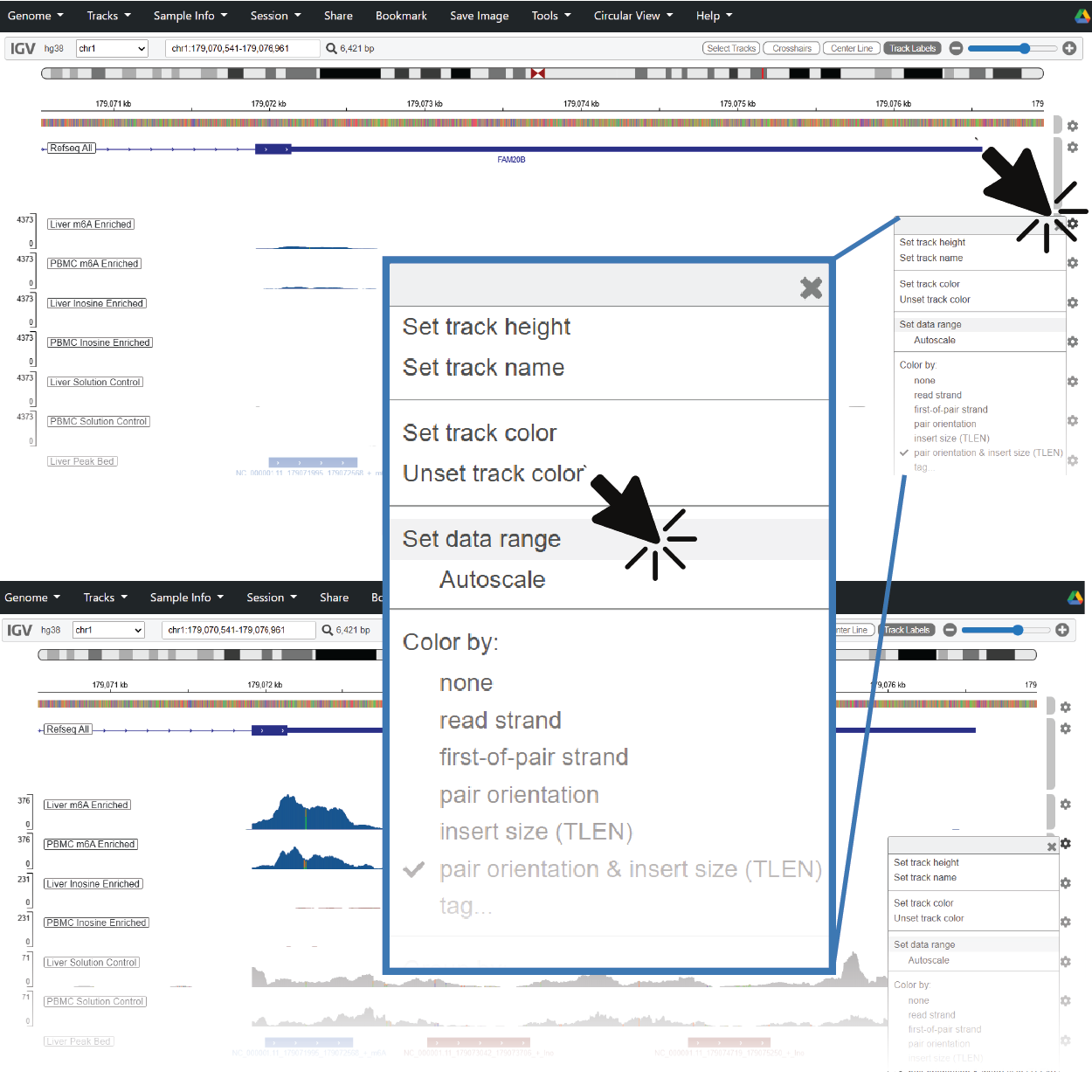
6. Check the Y-axis Scaling When You Navigate to Other Genes
Read counts for a given region of interest track proportionally with gene expression and have a wide dynamic range. If you don’t see any pileups, try rescaling the Y-axis.